Asymptotic Analysis and Upper Bounds

Recall our growth rates from a little while ago.

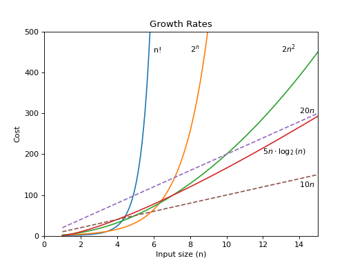
Despite the larger constant for the curve labeled \(10 n\) in the figure above, \(2 n^2\) crosses it at the relatively small value of \(n = 5\). What if we double the value of the constant in front of the linear equation? As shown in the graph, \(20 n\) is surpassed by \(2 n^2\) once \(n = 10\). The additional factor of two for the linear growth rate does not much matter. It only doubles the \(x\)-coordinate for the intersection point. In general, changes to a constant factor in either equation only shift where the two curves cross, not whether the two curves cross.

When you buy a faster computer or a faster compiler, the new problem size that can be run in a given amount of time for a given growth rate is larger by the same factor, regardless of the constant on the running-time equation. The time curves for two algorithms with different growth rates still cross, regardless of their running-time equation constants. For these reasons, we usually ignore the constants when we want an estimate of the growth rate for the running time or other resource requirements of an algorithm. This simplifies the analysis and keeps us thinking about the most important aspect: the growth rate. This is called asymptotic algorithm analysis. To be precise, asymptotic analysis refers to the study of an algorithm as the input size “gets big” or reaches a limit (in the calculus sense). However, it has proved to be so useful to ignore all constant factors that asymptotic analysis is used for most algorithm comparisons.

Big-O Notation

When trying to characterize an algorithm’s efficiency in terms of execution time, independent of any particular program or computer, it is important to quantify the number of operations or steps that the algorithm will require. If each of these steps is considered to be a basic unit of computation, then the execution time for an algorithm can be expressed as the number of steps required to solve the problem. Deciding on an appropriate basic unit of computation can be a complicated problem and will depend on how the algorithm is implemented.

Consider the problem of accumulating a sum. The idea of a simple loop to add values should be familiar.

accumulate1(int: N)
   sum ← 0
   count  ← N
   while count > 0
      sum ← sum + count
      count ← count - 1
   done while
   return sum
done accumulate

Compare the previous algorithm to this one:

accumulate2(int: N)
   if N ≡ 0 return N
   return N + accumulate(N-1)
done accumulate

Are both implementations valid?

Is one more efficient than the other?

How do we characterize functions that appear to be different and compare them using a consistent yardstick? Asymptotic analysis to the rescue.

A good basic unit of computation for comparing the summation algorithms shown earlier might be to count the number of assignment statements performed to compute the sum. In the function accumulate1, the number of assignment statements is 2 — assigning 0 to sum and assigning N to count, plus the value of n (the number of times we perform \(sum=sum+count\) and \(count=count-1\)). We can denote this by a function, call it T, where \(T(n)=2 + 2n\). The parameter n is often referred to as the “size of the problem,” and we can read this as “T(n) is the time it takes to solve a problem of size n, namely 2+2n steps.”

In the summation functions given above, it makes sense to use the number of terms in the summation to denote the size of the problem. We can then say that the sum of the first 100,000 integers is a bigger instance of the summation problem than the sum of the first 1,000. Because of this, it might seem reasonable that the time required to solve the larger case would be greater than for the smaller case. Our goal then is to show how the algorithm’s execution time changes with respect to the size of the problem.

Computer scientists prefer to take this analysis technique one step further. It turns out that the exact number of operations is not as important as determining the most dominant part of the \(T(n)\) function. In other words, as the problem gets larger, some portion of the \(T(n)\) function tends to overpower the rest. This dominant term is what, in the end, is used for comparison. The order of magnitude function describes the part of \(T(n)\) that increases the fastest as the value of n increases. Order of magnitude is often called Big-O notation (for “order”) and written as \(O(f(n))\). It provides a useful approximation to the actual number of steps in the computation. The function \(f(n)\) provides a simple representation of the dominant part of the original \(T(n)\).

In the above example, \(T(n)=2+2n\). As n gets large, the constants will become less and less significant to the final result. If we are looking for an approximation for \(T(n)\), then we can drop them and simply say that the running time is \(O(n)\). It is important to note that the constants are certainly significant for \(T(n)\). However, as n gets large, our approximation will be just as accurate without it.

Try This!

Prove to yourself that the recursive version of the summation in accumulate2 has the same \(O(n)\) performance as accumulate1.

Example

Suppose that for some algorithm, the exact number of steps is \(T(n)=5n^{2}+27n+1005\). When n is small, say 1 or 2, the constant 1005 seems to be the dominant part of the function. However, as n gets larger, the \(n^{2}\) term becomes the most important. In fact, when n is really large, the other two terms become insignificant in the role that they play in determining the final result. Again, to approximate \(T(n)\) as n gets large, we can ignore the other terms and focus on \(5n^{2}\). In addition, the coefficient \(5\) becomes insignificant as n gets large. We would say then that the function \(T(n)\) has an order of magnitude \(f(n)=n^{2}\), or simply that it is \(O(n^{2})\).

Self Check

sc-1-1: If the exact number of steps is \(T(n)=2n+3n^{2}-1\) what is the Big O?

• O(2n)
• No, 3n² dominates 2n. Try again.
• O(n)
• No, n² dominates n. Try again.
• O(3n²)
• No, the 3 should be omitted because n² dominates.
• O(n²)
• Right!
• More than one of the above
• No, only one of them is correct. Try again.

Without looking at the graph above, from top to bottom order the following from most to least efficient.

        constant
logarithmic
linear
log linear
quadratic
cubic
exponential
        

sc-1-3: Which of the following statements is true about the two algorithms? Algorithm 1: 100n + 1 Algorithm 2: n^2 + n + 1

• Algorithm 1 will require a greater number of steps to complete than Algorithm 2
• This could be true depending on the input, but consider the broader picture
• Algorithm 2 will require a greater number of steps to complete than Algorithm 1
• This could be true depending on the input, but consider the broader picture
• Algorithm 1 will require a greater number of steps to complete than Algorithm 2 until they reach the crossover point
• Correct!
• Algorithm 1 and 2 will always require the same number of steps to complete
• No, the efficiency of both will depend on the input

Using summation facts

Sometimes we can combine our knowledge of asymptotic analysis and math facts to make algorithms more efficient.

Starting with the original accumulate algortihm.

accumulate1(int: N)
   sum ← 0
   count  ← N
   while count > 0
      sum ← sum + count
      count ← count - 1
   done while
   return sum
done accumulate

When we discussed Summations, we saw that is loop is equivalent to

\[\sum_{k = 1}^{n} k = \frac{n (n+1)}{2}.\]

We can use this fact to transform our \(O(n)\) algorithm into \(O(1)\). The cost of \(O(1)\) algorithms is constant. Constant time algorithms do not grow more expensive as the size of \(n\) grows large.

#include <ctime> #include <iostream> clock_t start() { return clock(); } void time_since(clock_t start) { clock_t end = clock(); double elapsed_secs = double(end - start) / CLOCKS_PER_SEC; std::cout << std::fixed << " took "<< elapsed_secs << " seconds\n"; } long accumulate1(long n){ long sum = 0; for (long i = n; i > 0; --i){ sum = sum + i; } return sum; } long accumulate2(long n){ return (n*(n+1))/2; } int main(){ for (int N=1000; N<1e6; N*=10) { clock_t begin = clock(); std::cout << "N: " << N << ", Sum1 = " << accumulate1(N) << '\t'; time_since(begin); } for (int N=1000; N<1e6; N*=10) { clock_t begin = clock(); std::cout << "N: " << N << ", Sum2 = " << accumulate2(N) << '\t'; time_since(begin); } return 0; }

There are two important things to notice about this output. First, the times recorded above are shorter than any of the previous examples. Second, they are very consistent no matter what the value of \(n\). It appears that accumulate2 is hardly impacted by the number of integers being added.

But what does this benchmark really tell us? Intuitively, we can see that the iterative solutions seem to be doing more work since some program steps are being repeated. This is likely the reason it is taking longer. Also, the time required for the iterative solution seems to increase as we increase the value of \(n\). However, there is a problem. If we run the same function on a different computer or used a different programming language, we would get different results. It could take even longer to perform accumulate2 if the computer were older.

Asymptotic analysis gives us the tools to definitively state, without resorting to measuring execution time, that the accumulate2 runs in constant time, while the accumulate1 function runs in \(O(n)\) time.

Pitfall: Confusing upper bound and worst case

A common mistake people make is confusing the upper bound and worst case cost for an algorithm. The upper bound represents the highest growth rate an algorithm may have for size \(n\). The sequential search algorithm we discussed in Best, worst, and average cases involved 3 key input cases:

1. When the target value was in the first element (base case)

2. When the target value was not found (worst case)

3. The average cost for all possible locations, which works out to \(n/2\)

In the best case, only a single element is visited. Accordingly, the upper bound for this algorithm in the best case is \(O(1)\). Even when \(n\) grows large, the cost for the base case is constant.

In the worst case, every element is visited. Accordingly, the upper bound for this algorithm in the worst case is \(O(n)\). No matter the value of \(n\), for some constant \(c\), \(cn\) is bigger than \(n\).

In the average case, about \(\frac{n}{2}\) elements are visited. The upper bound for this algorithm in the average case is also \(O(n)\). As \(n\) grows large, the denominator becomes insignificant. No matter the value of \(n\), for some constant \(c\), \(cn\) is bigger than \(n/2\).

Therefore, question we should always consider is: what is the upper bound of our algorithm in the best / average / worst case? And the answer should be (sequential search):

• \(O(1)\) in the best case

• \(O(n)\) in the worst case

• \(O(n)\) in the average case

More to Explore

• TBD

Acknowledgements

This section is adapted from Problem Solving with Algorithms and Data Structures using C++, by Brad Miller and David Ranum, Luther College, and Jan Pearce, Berea College released under the CC BY-NC-SA 4.0.

You have attempted of activities on this page