16.3. Insertion sort

What would you do if you have a stack of phone bills from the past two years and you want to order by date? A fairly natural way to handle this is to look at the first two bills and put them in order. Then take the third bill and put it into the right position with respect to the first two, and so on. As you take each bill, you would add it to the sorted pile that you have already made. This simple approach is the inspiration for our first sorting algorithm, called Insertion Sort.

Insertion Sort iterates through a list of records. For each iteration, the current record is inserted in turn at the correct position within a sorted list composed of those records already processed. Given an array named data that stores \(n\) records, one way to implement an insertion sort could be this.

template <class Comparable>
void insertion_sort(Comparable* data[], int n) {
  for (int i = 1; i < n; ++i) {
    for (int j = i; (j > 0) && (*data[j] < *data[j-1]); --j) {
      swap(data, j, j-1);
     }
   }
}

This sort is still \(O(n^{2})\), but works differently from the bubble sort and selection sort, since it always maintains a sorted subvector in the container. Each new item is then “inserted” back into the previous subvector such that the sorted subvector is one item larger. Figure 4 shows the insertion sorting process. The shaded items represent the ordered subvectors as the algorithm makes each pass.

Figure 4: Insertion Sort

We begin by assuming that a vector with one item (position \(0\)) is already sorted. On each pass, one for each item 1 through \(n-1\), the current item is checked against those in the already sorted subvector. As we look back into the already sorted subvector, we shift those items that are greater to the right. When we reach a smaller item or the end of the subvector, the current item can be inserted.

Figure 5 shows the fifth pass in detail. At this point in the algorithm, a sorted subvector of five items consisting of 17, 26, 54, 77, and 93 exists. We want to insert 31 back into the already sorted items. The first comparison against 93 causes 93 to be shifted to the right. 77 and 54 are also shifted. When the item 26 is encountered, the shifting process stops and 31 is placed in the open position. Now we have a sorted subvector of six items.

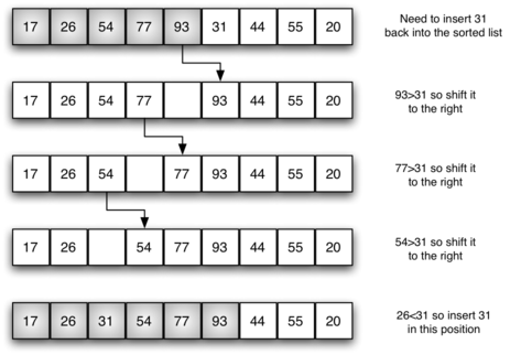
Figure 5: Insertion Sort: Fifth Pass of the Sort

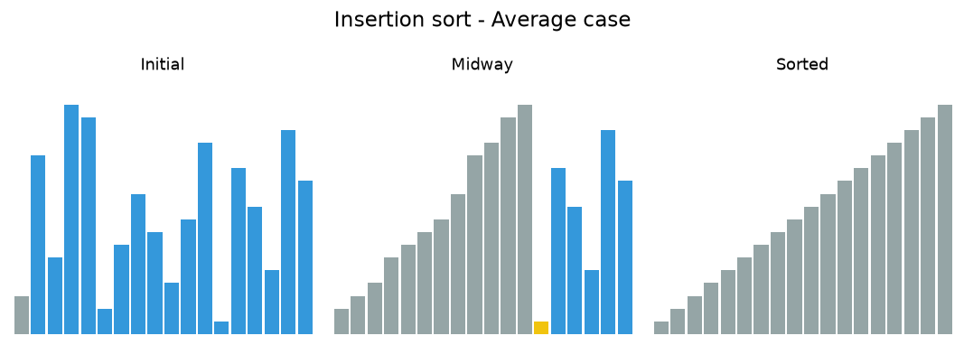
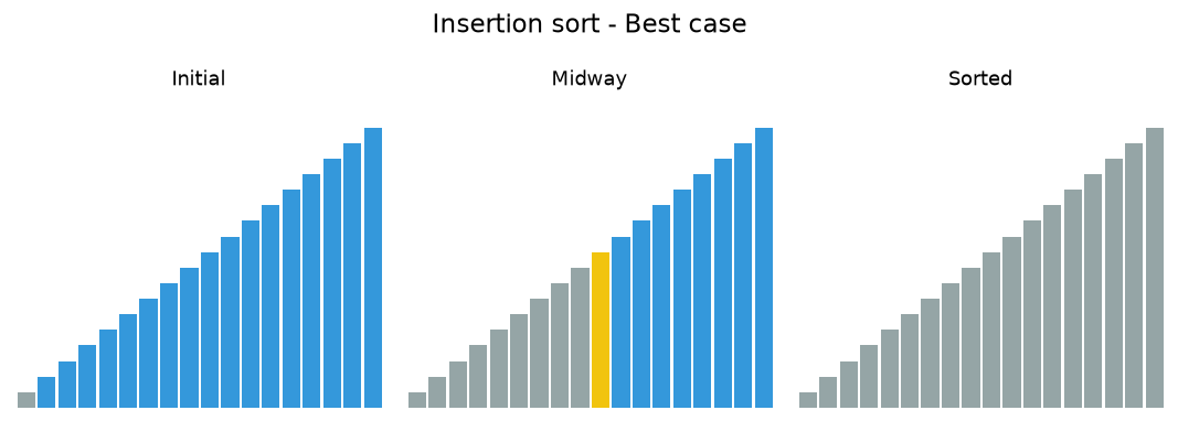
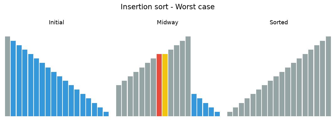
In the following animation, red bars represent the element being looked at and blue represents the last element to look at during a pass.

Initialize Run Stop
Beginning Step Forward Step Backward End

The implementation of insertion_sort (ActiveCode 1) shows that there are again \(n-1\) passes to sort n items. The iteration starts at position 1 and moves through position \(n-1\), as these are the items that need to be inserted back into the sorted subvectors. Line 8 performs the shift operation that moves a value up one position in the vector, making room behind it for the insertion. Remember that this is not a complete exchange as was performed in the previous algorithms.

The maximum number of comparisons for an insertion sort is the sum of the first \(n-1\) integers. Again, this is \(O(n^{2})\). However, in the best case, only one comparison needs to be done on each pass. This would be the case for an already sorted vector.

One note about shifting versus exchanging is also important. In general, a shift operation requires approximately a third of the processing work of an exchange since only one assignment is performed. In benchmark studies, insertion sort will show very good performance.

#include <iostream> #include <vector> using std::vector; vector<int> insertion_sort(vector<int> data) { for (unsigned int index=1; index<data.size(); ++index) { int currentvalue = data[index]; int position = index; while (position>0 && data[position-1]>currentvalue) { data[position] = data[position-1]; --position; } data[position] = currentvalue; } return data; } int main() { vector<int> data = {54, 26, 93, 17, 77, 31, 44, 55, 20}; for (const auto& value: insertion_sort(data)) { std::cout << value << ' '; } std::cout << '\n'; return 0; }

Self Check

sc-1-3: Suppose you have the following list of numbers to sort: [15, 5, 4, 18, 12, 19, 14, 10, 8, 20] which list represents the partially sorted list after three complete passes of insertion sort?

• [4, 5, 12, 15, 14, 10, 8, 18, 19, 20]
• This is the result of bubble sort.
• [15, 5, 4, 10, 12, 8, 14, 18, 19, 20]
• This is the result of selection sort.
• [4, 5, 15, 18, 12, 19, 14, 10, 8, 20]
• Insertion sort works at the start of the list. Each pass produces a longer sorted list.
• [15, 5, 4, 18, 12, 19, 14, 8, 10, 20]
• Insertion sort works on the front of the list not the end.

16.4. Costs of Exchange Sorting

The running time for each of the sorts discussed so far is \(\Theta(n^2)\) in the average and worst cases. The cost summary for the Insertion Sort, Bubble Sort, and Selection Sort in terms of their required number of comparisons and swaps in the best, average, and worst cases is shown.

\[\begin{split}\begin{array}{rccc} &\textbf{Insertion}&\textbf{Bubble}&\textbf{Selection}\\ \textbf{Comparisons:}\\ \textrm{Best Case}&\Theta(n)&\Theta(n^2)&\Theta(n^2)\\ \textrm{Average Case}&\Theta(n^2)&\Theta(n^2)&\Theta(n^2)\\ \textrm{Worst Case}&\Theta(n^2)&\Theta(n^2)&\Theta(n^2)\\ \\ \textbf{Swaps:}\\ \textrm{Best Case}&0&0&\Theta(n)\\ \textrm{Average Case}&\Theta(n^2)&\Theta(n^2)&\Theta(n)\\ \textrm{Worst Case}&\Theta(n^2)&\Theta(n^2)&\Theta(n)\\ \end{array}\end{split}\]

The remaining sorting algorithms presented in this chapter are significantly better than these three under typical conditions. But before continuing on, it is instructive to investigate what makes these three sorts so slow. The crucial bottleneck is that only adjacent records are compared. Thus, comparisons and moves (for Insertion and Bubble Sort) are by single steps. Swapping adjacent records is called an exchange. Thus, these sorts are sometimes referred to as an exchange sort. The cost of any exchange sort can be at best the total number of steps that the records in the array must move to reach their “correct” location. Recall that this is at least the number of inversions for the record. An inversion occurs when a record with key value greater than the current record’s key value appears before it.

More to Explore

• TBD

Acknowledgements

This section is adapted from Problem Solving with Algorithms and Data Structures using C++, by Brad Miller and David Ranum, Luther College, and Jan Pearce, Berea College released under the CC BY-NC-SA 4.0, and Open Data Structures (OpenDSA) by Ville Karavirta and Cliff Shaffer which is distributed under the MIT License.

You have attempted of activities on this page