15.1. Tree ADT concepts
If sequence containers like vector are so great, then why would we need anything else?
In a word: search.
When we have millions a elements in a data structure and need to find
just one element, or a specific range or elements,
we could use a vector.
Inserts are fast.
No matter how many elements are already in a vector
adding one more using push_back takes
the same amount of time.
That is, the time cost of push_back is constant for a vector.
A vector is default ordered only by its index position,
not by the values stored within it.
It's easy to keep throwing items in without paying any attention
to how they are ordered.
But always using push_back is analogous to a messy closet.
We could consider the closet to be ordered by depth:
the last things thrown in the closet are on the top of the pile.
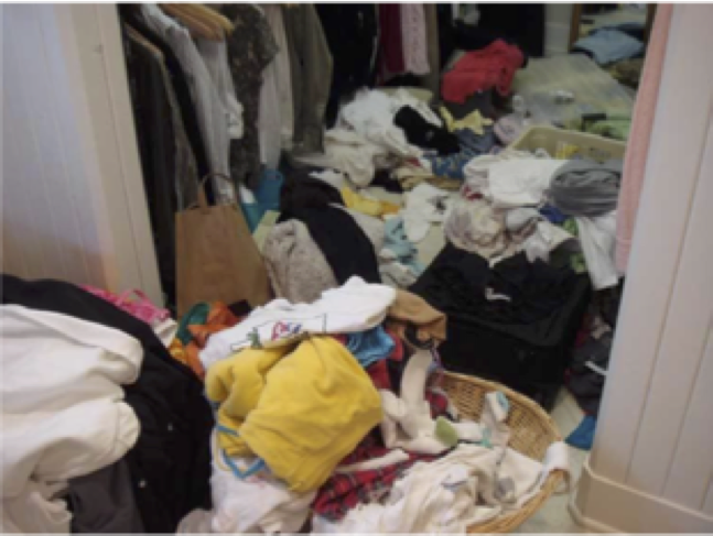
This makes getting a specific item from the closet slow. If we only ever want to to access the last item we added, then we know exactly where to go. But if we want to find some arbitrary item, we have to search the vector 1 element at a time until we find it.
vector<int> messy_closet (1024 * 1024 * 1024);  // a fairly big vector

// modify closet . . .

cout << "Go get some coffee while I work on this. . . \n";
for (const auto& v: messy_closet) {
  if (v == search_val) {
    do_something(v);
  }
}
Sometimes we may get lucky and find the desired element at index position 0. If the data added to the vector is random, then this becomes increasingly less likely as the size grows.
We might sometimes get very unlucky and not find the element until we access the last element. Over many searches, on average, we will have to examine \(N \over 2\) elements.
It's easy to see that the more elements are added, the longer searches will take.
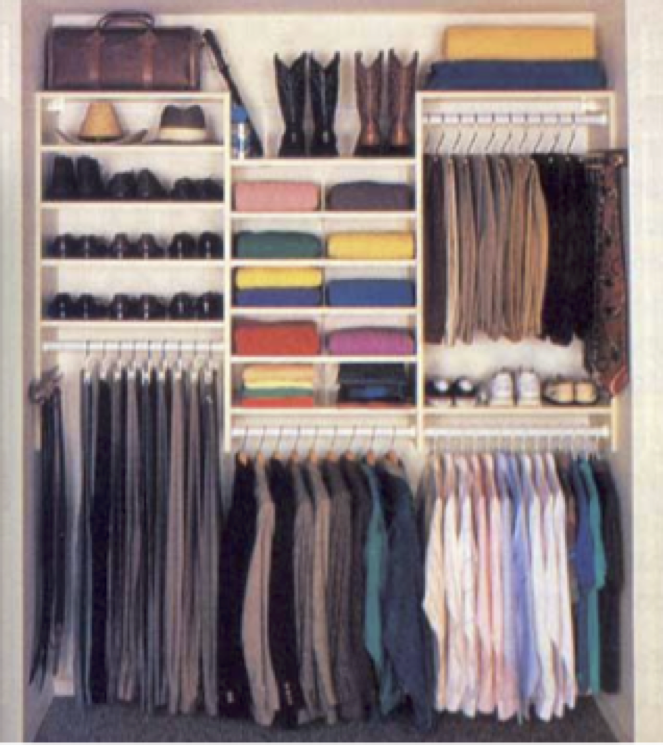
We need a tidy closet.
We could sort the vector, which would speed up our search.
The basic idea is to sort the vector,
then examine the value at position \(N \over 2\).
If the value found is greater than the value we are looking for,
then examine the value at position \(N \over 4\),
else examine the value at position \(3N \over 4\).
At each step,
we eliminate the number of remaining elements we need
to search in our vector by half.
For a large vector, this saves a lot of time.
This technique requires that we keep the vector sorted. If elements are added or removed frequently, then adding data to our vector, which used to be fast, is now slow. We can either use push_back followed by sort, or use insert. Every addition becomes a search and we are back to the original problem. On average, it will take \(N \over 2\) comparisons to add new data.
How can we solve this problem?
Can we make an ADT whose performance does not degrade as the number of elements in the ADT grows large?
Yes, but we need a new idea. Instead of a sequential container, we need a tree.
15.1.1. The tree ADT
A tree is a hierarchical abstract data type. Conceptually, it can be thought of as a collection of nodes defined by parent-child relationships.
One node is the root. It serves as the 'trunk' of the tree and serves the same function as the head of a list The root node is the only node in a tree without a parent. All other nodes in a tree refer to exactly 1 parent. In a binary tree, the children are commonly referred to as the left and right nodes.
Yes, programmers draw trees upside-down. The root is above the branches.
The height of a tree is the count of the nodes along the longest path in a tree from the root to a leaf node.
Although there are many different types of trees, we need only worry about binary trees. A binary tree is a tree in which no node has more than 2 children. Any tree node may have 0, 1, or 2 children. A tree node with no children is a leaf node.
All of these are valid binary trees:
A balanced tree (one with the roughly equal numbers of nodes in each subtree), provides the tidy room we need to ensure reasonably fast inserts and retrievals. A tree must be both balanced and sorted for us to gain benefits from a tree.
When a tree is balanced and sorted, the cost of both inserts and retrievals are on average \(log_2{N}\). Binary trees provide a way for us to 'formalize' our half-splitting solution.
Unbalanced trees are not much more than fancy linked lists. The performance of unbalanced trees degrades back to the messy room, with all of the problems and none of the benefits.
Balanced trees are the data structures that support both sets and maps.
More to Explore