16.5. Analysis of separate chaining
We define \(\lambda\), the load factor of a hash table, as the number of items contained in the table divided by the table size. Given a hash table with a separate bucket for each item to be stored and a well-behaved hash function, then \(\lambda = 1.0\) and the length of each list to also 1.
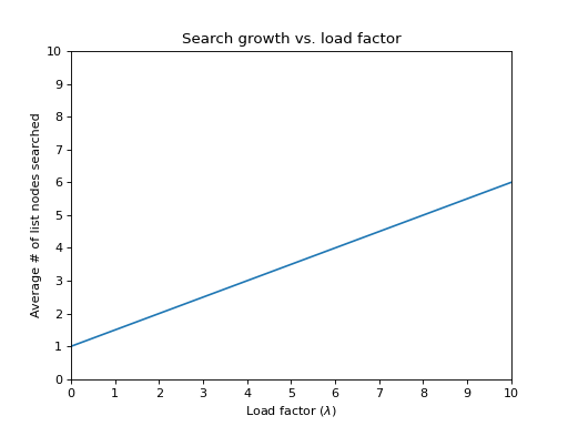
The effort required to perform a search is the constant time required to evaluate the hash function plus the time to traverse the list. In an unsuccessful search, the number of list nodes to examine is \(\lambda\) on average. A successful search requires that about \(1 + (\lambda / 2)\) links be traversed.
Why? Note that the list that is being searched contains the one node that stores the match plus zero or more other nodes The expected number of "other nodes" in a table of \(N\) elements and \(M\) lists is \((N - 1)/M = \lambda - 1/M\), which is essentially \(\lambda\), since \(M\) is often large. Recall our analysis of sequential data structures: on average, half the list is searched, so combined with the matching node, the average search cost is \(1 + \lambda / 2\) nodes. This shows that the table size is not nearly as important as the load factor. The general rule for separate chaining hashing is to make the table size about as large as the number of elements expected.
The graph shows how the cost of finding a node increases as \(\lambda\) increases.
In separate chaining hash tables suffer gradually declining performance as the load factor grows. There is no fixed point beyond which resizing is absolutely needed. Keep in mind that keeping the load factor < 1 in separate chaining may result in too many empty buckets. If memory is at a premium, we can trade some performance for space in memory.
If you are concerned about performance, then you should measure the load factor that maximizes performance on your system. Typically it will be between 1 and 3. One might think that \(\lambda = 1\) is the right place to rehash, but the best performance is often seen (for buckets implemented as linked lists) when load factors are in the 1 - 2 range.
If the load factor exceeds our threshold, then we expand the table size by calling rehash.
This process should also ensure the new hash table storage size maintain
a prime number of elements to ensure good distribution among buckets.
Note
For separate chaining, assuming a load factor of 1, this is one version of the classic balls and bins problem: Given \(N\) balls placed randomly (uniformly) in \(N\) bins, what is the expected number of balls in the most occupied bin?
The answer is known to be \(\theta \left ( \log{N}/\log {\log{N}} \right )\), meaning that on average, we expect some queries to take nearly logarithmic time. Similar types of bounds are observed (or provable) for the length of the longest expected probe sequence in a probing hash table. We would like to obtain \(O(1)\) worst-case cost.
Suppose we have inserted \(sz\) items into a table of size \(N\).
We could use a tree for each bucket,
which would reduce the cost of searching buckets to \(O(\log_{2}(sz))\)
with an extra cost that Key types support a operator< comparison
in addition to the operator== comparison required with list buckets.
In a list-based implementation, if N is much larger than sz,
and if our hash function uniformly distributes our keys,
then most lists will have 0 or 1 item,
and the average case is approximately \(O(1)\).
But if sz is much larger than N,
we are looking at an \(O(sz)\)
linear search sped up by a constant factor (N), but still \(O(sz)\).
Bottom line: hash tables let us trade space for speed.
More to Explore
Balls into bins problem on Wikipedia.