16.6. Closed hashing
In closed hashing, the hash array contains individual elements rather than a collection of elements. When a key we want to insert collides with a key already in the table, we resolve the collision by searching for another open slot within the table where we can place the new key.
Each slot in the hash table contains a hash_entry, composed of
one data element and a status field indicating whether that slot is
occupied, empty, or deleted.
hash_set
enum class hash_status { OCCUPIED, EMPTY, DELETED };

template <class T>
struct hash_entry
{
  T data;
  hash_status info;

  hash_entry(): info(hash_status::EMPTY)  {}
  hash_entry(const T& value, hash_status status)
    : data{value}
    , info(status)
    {}
};
The hash_set backing store is an array of hash_entry
objects.
template <class Key,
          size_t N,
          class Comparator=std::equal_to<Key>>
class hash_set
{
  public:
    using value_type = Key;
    using key_type   = Key;

    hash_set() = default;
  private:
    array<hash_entry<Key>, N> table;
    Comparator compare;
    size_t sz = 0;
};
Collisions are resolved by trying a series of locations, \(p_0, p_1, p_2, \ldots p_{N-1}\) until we find what we are looking for. Each position is calculated as:
where:
hash(value)is the home slotf()is a function taking an integer number of tries and returns an integer offset.
How are new positions used in the hash table?
- Searching:
Try positions \(p_0, p_1, p_2, \ldots\) until we find the requested value or an
EMPTYslot.- Inserting:
Try positions \(p_0, p_1, p_2, \ldots\) until we find the same value, an
EMPTYslot, or aDELETEDslot. Put the new value in the position pound and mark the position asOCCUPIED.- Erasing:
Try positions \(p_0, p_1, p_2, \ldots\) until we find the requested value or an
EMPTYslot. If we find the value, then mark the position asDELETED.
find
Find takes a value of the hash_entry key type as a parameter
and returns the position of the value in the table.
It returns N if the value is not in the table.
size_t find (const Key& value) const
{
  size_t hash = std::hash<Key>()(value);
  size_t pos = hash % N;
  size_t count = 0;
  while ((table[pos].info == hash_status::DELETED ||
         (table[pos].info == hash_status::OCCUPIED
         && (!compare(table[pos].data, value))))
      && count < N)
  {
    ++count;
    pos = (hash + next_slot(count)) % N;
  }
  if (count >= N || table[pos].info == hash_status::EMPTY) {
    return N;
  }
  return pos;
}
The loop condition is fairly complicated and needs discussion. There are three ways to exit this loop:
We hit an
EMPTYspace (notDELETED, and notOCCUPIED)We hit an
OCCUPIEDspace that has the value we wantWe have tried
Ndifferent positions. (No place left to look!)
contains
With find in place, other search operations are easy.
Simply call find and evaluate the results.
constexpr
  bool contains (const Key& value) const noexcept
{
  return  find(value) != N;
}

int count (const Key& value)
{
  unsigned pos = find(value);
  return  (pos == N) ? 0 : 1;
}
Note that since our set is still forcing a uniqueness constraint,
count will return only 0 or 1.
erase
The code to remove elements is just as simple.
Easier than the erase we implemented for open hashing.
We try to find that element.
If found, we mark that slot
DELETEDand decrement the size.Otherwise, do nothing.
void erase (const Key& value)
{
  unsigned pos = find(value);
  if (pos != N) {
    table[pos].info = hash_status::DELETED;
    --sz;
  }
}
insert
Inserts are a bit more work, because they involve potentially looking for an open slot to store a value.
Because this is a set (and not a multiset) we first call find
to see if the value is already there.
bool insert (const Key& value)
{
  size_t hash = std::hash<Key>()(value);
  unsigned pos = find(value);
  if (pos == N) {
    size_t count = 0;
    pos = hash % N;
    while (table[pos].info == hash_status::OCCUPIED && count < N)
    {
      ++count;
      pos = (hash + next_slot(count)) % N;
    }
    if (count >= N) {
      return false;  // could not add, table is full
    }
    table[pos].info = hash_status::OCCUPIED;
    table[pos].data = value;
    ++sz;
    return true;
  }
  // else replace existing value
  table[pos].data = value;
  return true;
}
If not found (pos == N), then we need to find a slot.
The loop that does this is similar the find loop,
but unlike find, we stop at the first DELETED or EMPTY slot.
In the other searches, we had kept going past DELETED slots,
because the element we wanted might have been stored
after an element that was later erased.
But now we are only looking for an unoccupied slot to put something,
so either a slot that has never been occupied (EMPTY) or
a slot that used to be occupied but is no longer (DELETED) works.
Run it
The example contains #define statements you can use to change
how the next slot is found.
Try it with different hash table sizes to see how clumping changes with the different probing strategies.
  1#include <array>
  2#include <cstddef>
  3#include <iomanip>
  4#include <iostream>
  5#include <utility>
  6
  7using std::array;
  8
  9#define USE_LINEAR_PROBING
 10
 11#if defined(USE_QUADRATIC_PROBING)
 12    // find next slot using quadratic probing
 13    constexpr
 14      size_t next_slot(size_t count) noexcept { return count*count; }
 15
 16#elif defined(USE_DOUBLE_HASHING)
 17
 18    // find next slot using double hashing
 19    constexpr
 20      size_t next_slot(size_t count) noexcept { return count * std::hash<size_t>()(count); }
 21#else   // default to USE_LINEAR_PROBING
 22    // find next slot using linear probing
 23    constexpr
 24      size_t next_slot(size_t count) noexcept { return count; }
 25
 26#endif
 27
 28
 29enum class hash_status { OCCUPIED, EMPTY, DELETED };
 30
 31template <class T>
 32struct hash_entry
 33{
 34  T data;
 35  hash_status info;
 36
 37  hash_entry(): info(hash_status::EMPTY)  {}
 38  hash_entry(const T& value, hash_status status)
 39    : data{value}
 40    , info(status)
 41    {}
 42};
 43
 44template <class T>
 45std::ostream& operator<<(std::ostream& os, const hash_entry<T>& rhs)
 46{
 47  if (rhs.info == hash_status::OCCUPIED) {
 48    os << rhs.data;
 49  } else if (rhs.info == hash_status::EMPTY) {
 50    os << 'E';
 51  } else {
 52    os << 'D';
 53  }
 54  return os;
 55}
 56
 57template <class Key,
 58         size_t N,
 59         class Comparator=std::equal_to<Key>>
 60class hash_set
 61{
 62  public:
 63    using value_type = Key;
 64    using key_type   = Key;
 65
 66    hash_set() = default;
 67
 68    size_t find (const Key& value) const
 69    {
 70      size_t hash = std::hash<Key>()(value);
 71      size_t pos = hash % N;
 72      size_t count = 0;
 73      while ((table[pos].info == hash_status::DELETED ||
 74             (table[pos].info == hash_status::OCCUPIED
 75             && (!compare(table[pos].data, value))))
 76          && count < N)
 77      {
 78        ++count;
 79        pos = (hash + next_slot(count)) % N;
 80      }
 81      if (count >= N || table[pos].info == hash_status::EMPTY) {
 82        return N;
 83      }
 84      return pos;
 85    }
 86
 87    constexpr
 88      bool contains (const Key& value) const noexcept
 89    {
 90      return  find(value) != N;
 91    }
 92
 93    int count (const Key& value)
 94    {
 95      unsigned pos = find(value);
 96      return  (pos == N) ? 0 : 1;
 97    }
 98
 99    void erase (const Key& value)
100    {
101      unsigned pos = find(value);
102      if (pos != N) {
103        table[pos].info = hash_status::DELETED;
104        --sz;
105      }
106    }
107
108
109    bool insert (const Key& value)
110    {
111      size_t hash = std::hash<Key>()(value);
112      unsigned pos = find(value);
113      if (pos == N) {
114        size_t count = 0;
115        pos = hash % N;
116        while (table[pos].info == hash_status::OCCUPIED && count < N)
117        {
118          ++count;
119          pos = (hash + next_slot(count)) % N;
120        }
121        if (count >= N) {
122          return false;  // could not add, table is full
123        }
124        table[pos].info = hash_status::OCCUPIED;
125        table[pos].data = value;
126        ++sz;
127        return true;
128      }
129      // else replace existing value
130      table[pos].data = value;
131      return true;
132    }
133
134
135    constexpr
136      size_t size() const noexcept { return sz; }
137
138    constexpr
139      bool empty() const noexcept { return sz == 0; }
140
141  private:
142    array<hash_entry<Key>, N> table;
143    Comparator compare;
144    size_t sz = 0;
145
146    friend
147      std::ostream& operator<<(std::ostream& os, const hash_set& rhs)
148      {
149        os << '[';
150        for (const auto& slot: rhs.table) {
151          os << slot << ',';
152        }
153        return os << ']';
154      }
155
156};
157
158int main() {
159  using std::cout;
160  using std::endl;
161  auto foo = hash_set<int, 11>{};
162  cout << "sz: " << foo.size() << endl;
163  cout << std::boolalpha << "mt?: " << foo.empty() << endl;
164  cout << foo << endl;
165  foo.insert(72);
166  foo.insert(72);
167  cout << "insert two 72's count:"<< endl;
168  cout << foo.count(72) << endl;
169  cout << foo << endl;
170  cout << "mt?: " << foo.empty() << endl;
171
172  foo.erase(72);
173  cout << "count after erase:"<< endl;
174  cout << foo.count(72) << endl;
175
176  foo.insert(-1);
177  foo.insert(0);
178  foo.insert(1);
179  foo.insert(2);
180  foo.insert(9);
181  foo.insert(81);
182  foo.insert(121);
183  foo.insert(572);
184  foo.insert(999);
185  cout << foo << endl;
186  foo.erase(-1);
187  cout << foo << endl;
188}
16.6.1. Choosing the next slot
The function next_slot(n) in the find and insert functions
controls the sequence of positions that will be checked.
It is the implementation of the function \(f(n)\) mentioned earlier.
Recall the find function:
size_t find (const Key& value) const
{
  size_t hash = std::hash<Key>()(value);
  size_t pos = hash % N;
  size_t count = 0;
  while ((table[pos].info == hash_status::DELETED ||
         (table[pos].info == hash_status::OCCUPIED
         && (!compare(table[pos].data, value))))
      && count < N)
  {
    ++count;
    pos = (hash + next_slot(count)) % N;
  }
  if (count >= N || table[pos].info == hash_status::EMPTY) {
    return N;
  }
  return pos;
}
On our \(n_{th}\) try, we examine the position
where \(hash(value)\) always returns the home slot for any
hashed value.
This is the location that the value would be stored if currently unoccupied.
The f function computes an offset from the reference location.
The most common schemes for choosing the next slot are
linear probing,
quadratic probing, and
double hashing.
- Linear probing
- \[f(n) = n\]
If a collision occurs at location
pos, we next check locations \(pos+1 \pmod N, pos+2 \pmod N, pos+3 \pmod N, \ldots\) and so on.Because collisions get stored in a location originally intended for another hash code, values have a tendency to clump together in the hash table.
- Quadratic probing
- \[f(n) = n^2\]
If a collision occurs at location
pos, we next check locations \(pos+1 \pmod N, pos+4 \pmod N, pos+9 \pmod N, \ldots\) and so on.Because the jumps between slots increases as the number of tries increases, this function tends to reduce clumping (and results in shorter searches). ``But`` it is not guaranteed to find an available empty slot if the table is more than half full or if
Nis not a prime number.Note
Again, prime numbers!
Remember the earlier discussion about how
% Ntends to improve the key distribution whenNis prime? You can see why it's part of programming "folklore" that hash tables should be prime-number sized, even if most programmers can't say why that's supposed to be good. - Double hashing
- \[f(n) = n * h_2(value)\]
where \(h_2\) is an alternate hash code function.
If a collision occurs at location
pos, we next check locations \((pos+1*h_2(value)) \pmod N, pos+2*h_2(value)) \pmod N, pos+3*h_2(value)) \pmod N, \ldots\) and so on.This also tends to reduce clumping, but, as with quadratic hashing, it is possible to get unlucky and miss open slots when trying to find a place to insert a new key.
16.6.2. Analysis of closed hashing
We define \(\lambda\), the load factor of a hash table, as the number of items contained in the table divided by the table size. In other words, the load factor measures what fraction of the table is full. By definition, \(0 \le \lambda \le 1\).
Given an ideal collision strategy, the probability of an arbitrary cell being full is \(\lambda\).
Therefore, the probability of an arbitrary cell being empty is \(1 - \lambda\).
The average number of table elements we expect to examine before finding an open position is therefore \(\frac {1}{1-\lambda}\).
Since we never look at more than N positions,
given an ideal collision strategy, finds and inserts are on average
The graph shows how \(\frac {1}{1-\lambda}\) changes as \(\lambda\) increases.
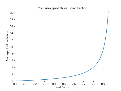
If the table is less than half full (\(\lambda < 0.5\))
then we expect to try on average no more than 2 slots
during a search or insert.
Not too bad.
But as \(\lambda\) gets larger,
the average number of slots examined grows toward N.
As the table fills and sz approaches N, the performance
degenerates toward \(O(N)\) behavior.
Because of this, a general rule of thumb for hash tables is to keep them no more than half full. At that load factor, we can treat searches and inserts as \(O(1)\) operations. If we let the load factor get much higher, we start seeing \(O(N)\) performance.
No collision resolution scheme is truly ideal, so keeping the load factor low enough is even more important in practice than this idealized analysis indicates.
More to Explore
The content on this page was adapted from Resolving Collisions <https://www.cs.odu.edu/~zeil/cs361/f25-web/Public/collisions/index.html>, by Steven J. Zeil for his data structures course CS361.