7.6. Merge sort

We now turn our attention to using a divide and conquer strategy as a way to improve the performance of sorting algorithms. The first algorithm we will study is the merge sort. Merge sort is a recursive algorithm that continually splits a vector in half. If the vector is empty or has one item, it is sorted by definition (the base case). If the vector has more than one item, we split the vector and recursively invoke a merge sort on both halves. Once the two halves are sorted, the fundamental operation, called a merge, is performed. Merging is the process of taking two smaller sorted vectors and combining them together into a single, sorted, new vector. Figure 10 shows our familiar example vector as it is being split by mergeSort. Figure 11 shows the simple vectors, now sorted, as they are merged back together.

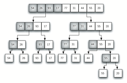
Figure 10: Splitting the vector in a Merge Sort

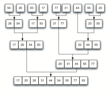
Figure 11: vectors as They Are Merged Together

Merge Sort

The merge_sort function begins by checking the base case. If the length of the vector is less than or equal to one, then we already have a sorted vector and no more processing is needed. If the length is greater than one, then we extract the left and right halves. It is important to note that the vector may not have an even number of items. That does not matter, as the lengths will differ by at most one.

Once the merge_sort function is invoked on the left half and the right half (lines 23-24), it is assumed they are sorted. The rest of the function is responsible for merging the two smaller sorted vectors into a larger sorted vector. Notice that the merge operation places the items back into the original vector (data) one at a time by repeatedly taking the smallest item from the sorted vectors.

The print function shows the vector contents at the start of each invocation. There is also a print call at the end to show the merging process. The output shows the result of executing the function on our example vector.

Note that the vector with 44, 55, and 20 will not divide evenly. The first split gives [44] and the second gives [55,20]. It is easy to see how the splitting process eventually yields a vector that can be immediately merged with other sorted vectors.

Run It

The Merge Sort

#include <iostream>
#include <string>
#include <vector>
using std::cout;
using std::vector;

void print(const vector<int>& data) {
   for (const auto& value: data) {
      cout << value << ' ';
   }
   cout << '\n';
}

vector<int> merge_sort(vector<int> data) {
   cout << "Splitting ";
   print(data);
   if (data.size() > 1) {
      int mid = data.size() / 2;
      // split data into 2 halves
      vector<int> left(data.begin(),data.begin()+mid);
      vector<int> right(data.begin()+mid,data.end());

      left = merge_sort(left);
      right = merge_sort(right);

      int i = 0, j = 0, k = 0;
      while (i < int(left.size()) && j < int(right.size())) {
         if(left[i] < right[j]) {
            data[k] = left[i];
            ++i;
         } else {
            data[k] = right[j];
            ++j;
         }
         ++k;
      }
      while(i < int(left.size())) {
         data[k] = left[i];
         ++i;
         ++k;
      }
      while(j < int(right.size())) {
         data[k] = right[j];
         ++j;
         ++k;
      }
   }
   cout << "Merging ";
   print(data);

   return data;
}

int main() {
  vector<int> data = {54, 26, 93, 17, 77, 31, 44, 55, 20};
  print(merge_sort(data));
  return 0;
}

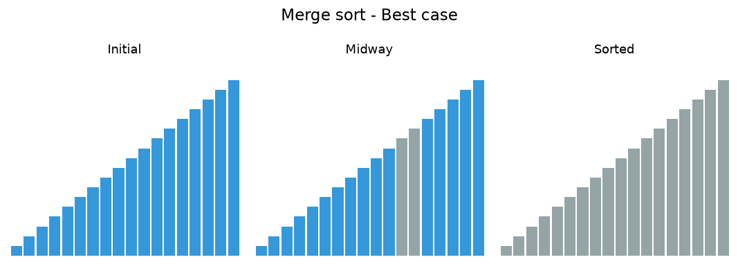
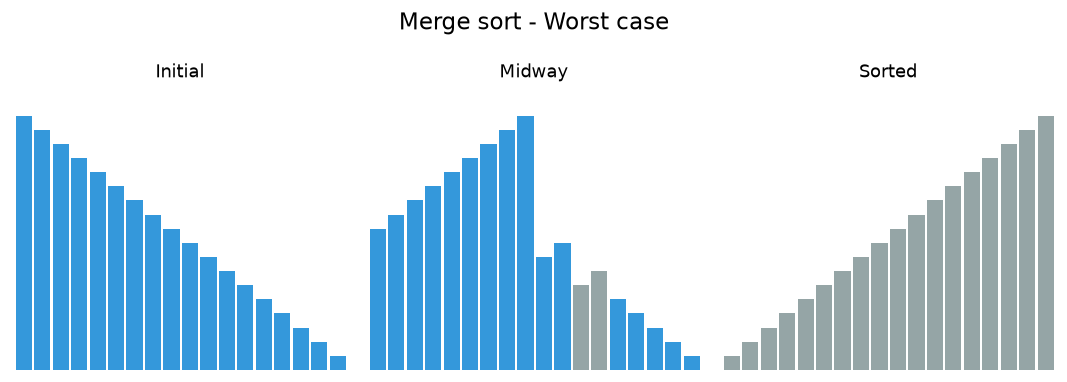
In the following animations, purple marks a range being split, teal marks the range being merged, yellow marks the target slot currently filled, and gray marks merged ranges.

Average case

Open video

Best case

Open video

Worst case

Open video

7.6.1. Merge sort analysis

In order to analyze the merge_sort function, we need to consider the two distinct processes that make up its implementation. First, the vector is split into halves. We already computed (in a binary search) that we can divide a vector in half \(\log n\) times where n is the length of the vector. The second process is the merge. Each item in the vector will eventually be processed and placed on the sorted vector. So the merge operation which results in a vector of size n requires n operations. The result of this analysis is that \(\log n\) splits, each of which costs \(n\) for a total of \(n\log n\) operations. A merge sort is an \(O(n \cdot log n)\) algorithm and even better, it is also \(\Omega(n \cdot log n)\) in the worst case.

Recall that the slicing operator is \(O(k)\) where k is the size of the slice. In order to guarantee that merge_sort will be \(O(n \cdot log n)\) we will need to remove the slice operator. Again, this is possible if we simply pass the starting and ending indices along with the vector when we make the recursive call. We leave this as an exercise.

It is important to notice that the merge_sort function requires extra space to hold the two halves as they are extracted with the slicing operations. This additional space can be a critical factor if the vector is large and can make this sort problematic when working on large data sets.

Self Check

Q1

Given the following list of numbers: [21, 1, 26, 45, 29, 28, 2, 9, 16, 49, 39, 27, 43, 34, 46, 40] which answer illustrates the list to be sorted after 3 recursive calls to mergesort?

[16, 49, 39, 27, 43, 34, 46, 40]

This is the second half of the list.

[21,1]

Yes, mergesort will continue to recursively move toward the beginning of the list until it hits a base case.

[21, 1, 26, 45]

Remember mergesort doesn't work on the right half of the list until the left half is completely sorted.

[21]

This is the list after 4 recursive calls

Check answer

Q2

Given the following list of numbers: [21, 1, 26, 45, 29, 28, 2, 9, 16, 49, 39, 27, 43, 34, 46, 40] which answer illustrates the first two lists to be merged?

[21, 1] and [26, 45]

The first two lists merged will be base case lists, we have not yet reached a base case.

[[1, 2, 9, 21, 26, 28, 29, 45] and [16, 27, 34, 39, 40, 43, 46, 49]

These will be the last two lists merged

[21] and [1]

The lists [21] and [1] are the first two base cases encountered by mergesort and will therefore be the first two lists merged.

[9] and [16]

Although 9 and 16 are next to each other they are in different halves of the list starting with the first split.

Check answer

More to Explore

• TBD

Acknowledgements

This section is adapted from Problem Solving with Algorithms and Data Structures using C++, by Brad Miller and David Ranum, Luther College, and Jan Pearce, Berea College released under the CC BY-NC-SA 4.0.