16.7. Quick sort¶

The quick sort uses divide and conquer to gain the same advantages as the merge sort, while not using additional storage. As a trade-off, however, it is possible that the list may not be divided in half. When this happens, we will see that performance is diminished.

A quick sort first selects a value, which is called the pivot value. Although there are many different ways to choose the pivot value, we will simply use the first item in the list. The role of the pivot value is to assist with splitting the list. The actual position where the pivot value belongs in the final sorted list, commonly called the split point, will be used to divide the list for subsequent calls to the quick sort.

Figure 12 shows that 54 will serve as our first pivot value. Since we have looked at this example a few times already, we know that 54 will eventually end up in the position currently holding 31. The partition process will happen next. It will find the split point and at the same time move other items to the appropriate side of the list, either less than or greater than the pivot value.

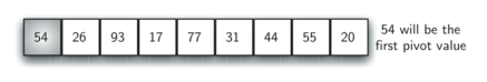
../_images/firstsplit.png — Figure 12: The First Pivot Value for a Quick Sort¶

Partitioning begins by locating two position markers—let’s call them leftmark and rightmark—at the beginning and end of the remaining items in the list (positions 1 and 8 in Figure 13). The goal of the partition process is to move items that are on the wrong side with respect to the pivot value while also converging on the split point. Figure 13 shows this process as we locate the position of 54.

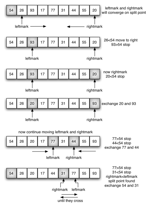
../_images/partitionA.png — Figure 13: Finding the Split Point for 54¶

We begin by incrementing leftmark until we locate a value that is greater than the pivot value. We then decrement rightmark until we find a value that is less than the pivot value. At this point we have discovered two items that are out of place with respect to the eventual split point. For our example, this occurs at 93 and 20. Now we can exchange these two items and then repeat the process again.

At the point where rightmark becomes less than leftmark, we stop. The position of rightmark is now the split point. The pivot value can be exchanged with the contents of the split point and the pivot value is now in place (Figure 14). In addition, all the items to the left of the split point are less than the pivot value, and all the items to the right of the split point are greater than the pivot value. The list can now be divided at the split point and the quick sort can be invoked recursively on the two halves.

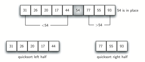
../_images/partitionB.png — Figure 14: Completing the Partition Process to Find the Split Point for 54¶

The partition function implements the process described earlier. The following program sorts the list that was used in the example above.

#include <iostream>
#include <string>
#include <utility>
#include <vector>
using std::vector;

void print(const vector<int>& data) {
   for (const auto& value: data) {
      std::cout << value << ' ';
   }
   std::cout << '\n';
}

int partition (vector<int>& data, int first, int last) {
   int pivotvalue = data[first];
   int rightmark = last;
   int leftmark = first + 1;
   bool done = false;
   while (!done) {
      while(leftmark <= rightmark &&
            data[leftmark] <= pivotvalue) {
        ++leftmark;
      }
      while(rightmark >= leftmark &&
            data[rightmark] >= pivotvalue) {
        --rightmark;
      }
      if(rightmark<leftmark) {
         done = true;
      } else {
         std::swap(data[rightmark], data[leftmark]);
      }
   }
   std::swap(data[rightmark], data[first]);
   return rightmark;
}

vector<int> quick_sort(vector<int>& data, int first, int last) {
   int pivot = 0;

if (first < last) {
      pivot = partition(data, first, last);
      quick_sort(data, first, pivot);
      quick_sort(data, pivot+1, last);
   }
   return data;
}

int main() {
  vector<int> data = {54, 26, 93, 17, 77, 31, 44, 55, 20};
  print(quick_sort(data, 0, data.size()-1));
  return 0;
}

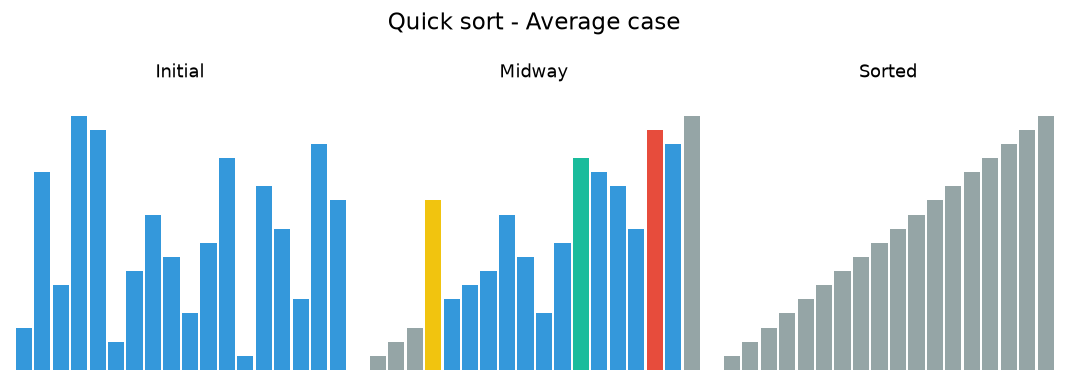
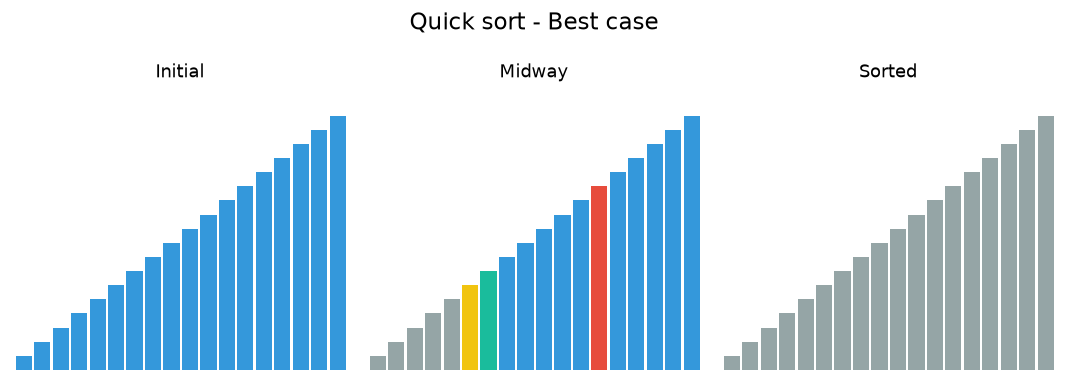
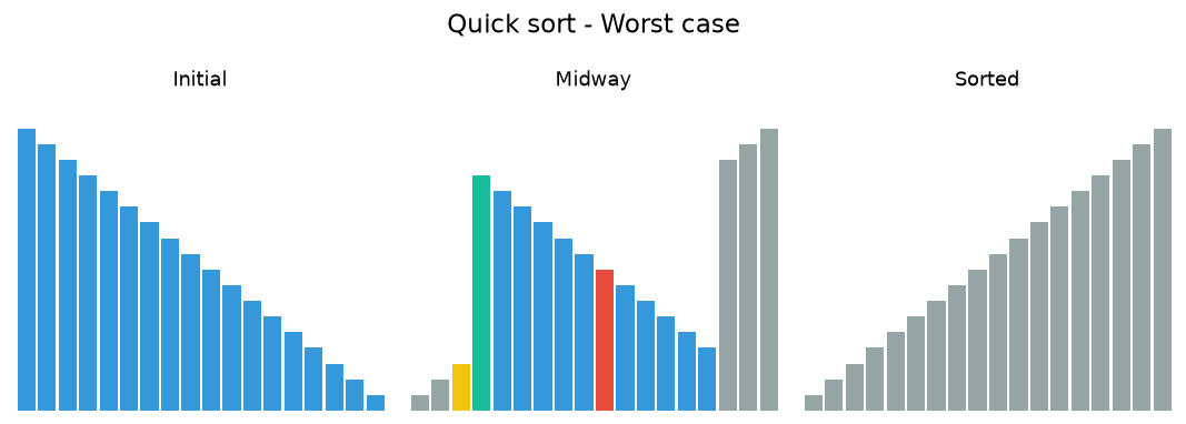
The following animation shows the quick sort in action. Our pivot is represented by the arrow on screen. If an object is bigger than the pivot, it will turn blue and stay where it is. If it is smaller it will turn red and swap to the left side of the pivot. Once an object is sorted, it will turn yellow.

The visualization above shows how quick sort works in action. Our pivot is represented by the arrow on screen. If an object is bigger than the pivot, it will turn blue and stay where it is. If it is smaller it will turn red and swap to the left side of the pivot. Once an object is sorted, it will turn yellow.

To analyze the quick_sort function, note that for a list of length n, if the partition always occurs in the middle of the list, there will again be \(\log n\) divisions. In order to find the split point, each of the n items needs to be checked against the pivot value. Therefore, the average case complexity is \(n\cdot \log n\). In addition, there is no copying of list data as in the merge sort process.

Unfortunately, in the worst case, the split points may not be in the middle and can be very skewed to the left or the right, leaving a very uneven division. In this case, sorting a list of n items divides into sorting a list of 0 items and a list of \(n-1\) items. Then sorting a list of \(n-1\) divides into a list of size 0 and a list of size \(n-2\), and so on. The result is an \(O(n^{2})\) sort with all of the overhead that recursion requires.

A recursive \(O(n^{2})\) algorithm makes quick sort susceptible to stack overflow errors on very large data sets.

Quick sort therefore poses an interesting dilemma. The quick sort average case is very fast. It tends to be the fastest, on average, of the known \(O(n \cdot log{n})\) average case sorting algorithms in actual clock time. But its worst case is just dreadful.

So the suitability of quick sort winds up coming down to a question of how often we would actually expect to encounter the worst case or nearly worst case behavior. That, in turn, depends upon the choice of pivot.

We mentioned earlier that there are different ways to choose the pivot value. In particular, we can attempt to alleviate some of the potential for an uneven division by using a technique called median of three. To choose the pivot value, we will consider the first, the middle, and the last element in the list. In our example, those are 54, 77, and 20. Now pick the median value, in our case 54, and use it for the pivot value (of course, that was the pivot value we used originally). The idea is that in the case where the first item in the list does not belong toward the middle of the list, the median of three will choose a better “middle” value. This will be particularly useful when the original list is somewhat sorted to begin with. We leave the implementation of this pivot value selection as an exercise.

Self Check

sc-1-3: Given the following list of numbers [14, 17, 13, 15, 19, 10, 3, 16, 9, 12] which answer shows the contents of the list after the second partitioning according to the quicksort algorithm?

[9, 3, 10, 13, 12]
It's important to remember that quicksort works on the entire list and sorts it in place.
[9, 3, 10, 13, 12, 14]
Remember quicksort works on the entire list and sorts it in place.
[9, 3, 10, 13, 12, 14, 17, 16, 15, 19]
The first partitioning works on the entire list, and the second partitioning works on the left partition not the right.
[9, 3, 10, 13, 12, 14, 19, 16, 15, 17]
The first partitioning works on the entire list, and the second partitioning works on the left partition.

sc-1-4: Given the following list of numbers [1, 20, 11, 5, 2, 9, 16, 14, 13, 19] what would be the first pivot value using the median of 3 method?

1
The three numbers used in selecting the pivot are 1, 9, 19. 1 is not the median, and would be a very bad choice for the pivot since it is the smallest number in the list.
9
Good job.
16
although 16 would be the median of 1, 16, 19 the middle is at len(list) // 2.
19
the three numbers used in selecting the pivot are 1, 9, 19. 9 is the median. 19 would be a bad choice since it is almost the largest.

sc-1-5: Which of the following sort algorithms are guaranteed to be O(n log n) even in the worst case?

Shell Sort
Shell sort is between O(n) and O(n^2)
Quick Sort
Quick sort can be O(n log n), but if the pivot points are not well chosen and the list is just so, it can be O(n^2).
Merge Sort
Merge Sort is the only guaranteed O(n log n) even in the worst case. The cost is that merge sort uses more memory.
Insertion Sort
Insertion sort is O(n^2)

sc-1-6: Match each sorting method with its appropriate estimated comparisons.

Refer to previous sections of the chapter

Quick Sort
O(n log n) or O(n^2)
Insertion/Bubble/Merge
O(n^2)
Merge Sort
O(n log n)
Shell Sort
between O(n) and O(n^2)

sc-1-7: Which sort should you use for best efficiency if you need to sort through 100,000 random items in a list?

Merge
Correct!
Selection
Selection sort is inefficient in large lists.
Bubble
Bubble sort works best with mostly sorted lists.
Insertion
Insertion sort works best with either small or mostly sorted lists.

More to Explore

You have attempted of activities on this page